---
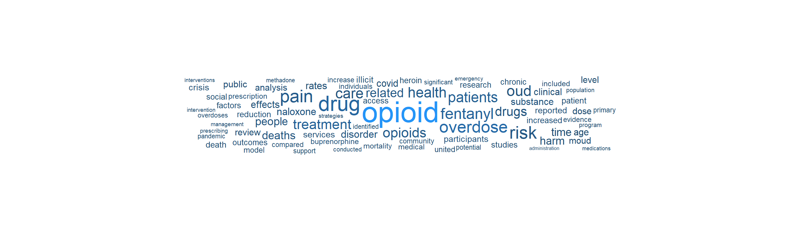
title: "The U.S. Drug Overdose Crisis"
author: "André van Zyl, MPH"
date-modified: today
---
# The U.S. Drug Overdose Crisis
The United States stands alone among high-income nations in the scale of its overdose crisis. Drug overdoses claimed more than 100,000 lives for a third consecutive year in 2023, representing over a 50 percent increase since 2019 [@commonwealth_overdose_intl]. With an overdose rate of 324 deaths per million people (nearly 108,000 deaths in 2022), the U.S. has by far the highest overdose death rate in the world. While Scotland and Canada, the next highest-ranked countries, saw declines from 2021 to 2022, rates in the U.S. have remained persistently elevated [@commonwealth_overdose_intl].
According to the [CDC National Center for Health Statistics](https://www.cdc.gov/nchs/fastats/leading-causes-of-death.htm), the three leading causes of death in the U.S. are heart disease (680,981 deaths), cancer (613,352), and unintentional injuries (222,698), with drug poisonings dominating the latter category [@cdc_faststats]. Drug overdose has become a [leading cause of injury mortality](https://www.cdc.gov/nchs/hus/topics/drug-overdose-deaths.htm), with opioids driving an increasing share of these deaths since 2009 and accounting for over 70% of all overdose fatalities [@cdc_hus_overdose]. The growing involvement of stimulants such as cocaine and methamphetamine alongside opioids has further complicated the crisis, transforming what began as a prescription opioid problem into a polysubstance mass-casualty event.
No peer nation experiences anything comparable. The [Commonwealth Fund 2025 Scorecard on State Health System Performance](https://www.commonwealthfund.org/publications/scorecard/2025/jun/2025-scorecard-state-health-system-performance) documents that premature, avoidable deaths are increasing in the United States while declining in comparable high-income countries, with drug overdose a major contributor to this divergence [@commonwealth2025]. The rate of avoidable mortality in West Virginia is more than twice the rate in Massachusetts, and wide racial disparities in premature deaths are the norm in most states [@commonwealth2025]. While overdose deaths fell slightly between 2022 and 2023 in 37 states, the total remains above 100,000 annually, and rates spiked by 25% or more in Nevada, Oregon, Washington, and Alaska [@commonwealth2025].
This chapter explores what the data shows, where the crisis hits hardest, and how to access and analyze the underlying datasets and research literature programmatically.
::: {.callout-tip title="Interactive Dashboard"}
An interactive companion dashboard, the [Drug Overdose Crisis Explorer](https://intersect-collaborations-llc.shinyapps.io/drug-overdose-explorer/), accompanies this chapter. It integrates the same six data sources covered below into a single R Shiny application with on-demand data loading, interactive visualizations, and Excel downloads with clickable links to source records. All source code for both this chapter and the dashboard is publicly available on [GitHub](https://github.com/andre-inter-collab-llc/Public_Health_Analytics_Playbook).
:::
## Why This Chapter
My path to this topic stems from my educational background and professional experience. I studied psychology and counseling in South Africa, where I worked as a supportive counselor at a residential recovery center for people with substance use disorders. That experience gave me a ground-level understanding of addiction, recovery, and the human cost of substance-related harm.
When I moved to the United States, I helped with the development of COVID-19 contact tracing systems before joining a local health department as an epidemiologist, where my responsibilities included drug overdose mortality monitoring and surveillance. I worked with county-level data coming from different jurisdictions, most of which was not programmatically accessible. After working at the health department, I continued at the CDC on COVID-19 response work and then antimicrobial resistance (AMR) response, but the opioid epidemic never left my peripheral vision.
Now, with more capacity to investigate, I am returning to the overdose landscape with fresh analytical tools and a broader perspective. As the published literature documents, the scale of drug overdose mortality in the United States is without parallel among high-income nations [@commonwealth2025]. This chapter is my attempt to understand the current state of the crisis: to see what data is available, to assess the impact and scale, to trace where funding is flowing, to examine what interventions are being tried, and to survey the research being conducted in the field.
## The Scale of the Problem
Drug overdose deaths in the United States have followed a steep, accelerating trajectory over the past 25 years. Approximately 105,000 people died from drug overdose in 2023, with nearly 80,000 (76%) of those deaths involving opioids. The number of opioid overdose deaths in 2023 was nearly ten times the number in 1999, though 2023 marked the first annual decline since 2018 [@cdc_opioid_epidemic]. From 1999 to 2023, approximately 806,000 people died from an opioid overdose in the United States [@cdc_opioid_epidemic].
The [CDC describes three distinct waves](https://www.cdc.gov/overdose-prevention/about/understanding-the-opioid-overdose-epidemic.html) of opioid overdose deaths [@cdc_opioid_epidemic]:
1. **Wave 1 (1990s)**: Increased prescribing of opioids drove a rise in overdose deaths involving prescription opioids (natural and semi-synthetic opioids and methadone) starting around 1999, though these have declined in recent years
2. **Wave 2 (2010)**: Rapid increases in overdose deaths involving heroin began in 2010, though heroin overdose deaths have also been declining in recent years
3. **Wave 3 (2013 onward)**: Substantial increases in overdose deaths involving synthetic opioids, particularly illegally manufactured fentanyls (IMFs), which have largely saturated the illegal drug supply
The third wave remains the dominant driver. IMFs are found in powder form or pressed into counterfeit pills and frequently contain other drugs, including non-opioid sedatives such as xylazine [@cdc_opioid_epidemic]. From 2022 to 2023, the rate of overdose deaths involving synthetic opioids decreased approximately 2%, heroin deaths decreased roughly 33%, and prescription opioid deaths decreased nearly 12% [@cdc_opioid_epidemic]. Despite these declines, in 2023, nearly 47% of drug overdose deaths involved both opioids and stimulants, underscoring the polysubstance nature of the current crisis [@cdc_opioid_epidemic]. Data from the [SUDORS Dashboard](https://www.cdc.gov/overdose-prevention/data-research/facts-stats/sudors-dashboard-fatal-overdose-data.html) further confirms this pattern: in 2024, 73.4% of overdose deaths involved at least one opioid and 65.1% involved at least one stimulant [@cdc_sudors]. Critically, 67.5% of overdose deaths had at least one potential opportunity for intervention, and in 2022, 77% of adults with substance use disorder were not receiving treatment [@commonwealth2025].
## Data Sources
The primary datasets for analyzing drug overdose mortality in the United States are:
### CDC WONDER
[CDC WONDER](https://wonder.cdc.gov/) (Wide-ranging ONline Data for Epidemiologic Research) is the premier federal system for querying mortality data from the National Vital Statistics System. It provides:
- Mortality counts, crude rates, and age-adjusted rates
- Stratification by geography (national, state, county), demographics, urbanization, and ICD-10 codes
- Multiple Cause of Death files that capture all substances listed on the death certificate
::: {.callout-warning title="Data Suppression"}
CDC WONDER suppresses counts below 10 deaths in any given cell to prevent identification. Analyses of small populations or rare drug categories at the county level will encounter this limitation.
:::
### CDC Open Data (WONDER API and Socrata)
CDC publishes several overdose-specific datasets on its open data portal at [data.cdc.gov](https://data.cdc.gov/), including provisional drug overdose death counts updated monthly. These datasets are Socrata-hosted and accessible via API.
### State and Local Portals
Many states and local jurisdictions maintain their own open data portals with overdose-related datasets, often including more granular geographic or toxicological detail than federal sources. These vary in format, update frequency, and accessibility, but are worth exploring for jurisdiction-specific analyses.
## Accessing the Data with R
### VSRR Provisional Drug Overdose Death Counts
The primary dataset used in this chapter is the [VSRR Provisional Drug Overdose Death Counts](https://data.cdc.gov/NCHS/VSRR-Provisional-Drug-Overdose-Death-Counts/xkb8-kh2a) (dataset ID: `xkb8-kh2a`), published by the [National Center for Health Statistics (NCHS)](https://www.cdc.gov/nchs/nvss/vsrr/drug-overdose-data.htm) as part of the Vital Statistics Rapid Release (VSRR) program [@ahmad_vsrr_2026]. This dataset presents provisional counts of drug overdose deaths based on the current flow of mortality data in the [National Vital Statistics System (NVSS)](https://www.cdc.gov/nchs/nvss/index.htm). It is updated monthly, with data available within four months after the date of death.
Provisional counts may not include all deaths that occurred during a given period because drug overdose deaths often require lengthy investigation, including toxicology testing. Death certificates may initially be filed with manner of death "pending investigation" or with a preliminary cause of death. To address this undercount, NCHS developed statistical methods to generate **predicted provisional counts** that adjust for reporting delays based on historical completeness patterns [@ahmad_vsrr_2026]. Drug overdose deaths are identified using ICD-10 underlying cause-of-death codes: X40--X44 (unintentional), X60--X64 (suicide), X85 (homicide), and Y10--Y14 (undetermined intent).
The dataset reports **12-month ending counts**, meaning each row represents the total number of deaths occurring in the 12-month period ending in the month indicated. For example, a row for June 2024 captures deaths from July 2023 through June 2024. This rolling window smooths out seasonal variation and provides a stable trend measure. The `indicator` field specifies which outcome is being counted: total drug overdose deaths, or deaths involving a specific drug or drug class, identified by ICD-10 multiple cause-of-death codes:
- **Heroin** (T40.1)
- **Natural opioid analgesics** including morphine, codeine, oxycodone, hydrocodone (T40.2)
- **Methadone** (T40.3)
- **Synthetic opioids other than methadone**, including fentanyl and tramadol (T40.4)
- **Cocaine** (T40.5)
- **Psychostimulants with abuse potential**, including methamphetamine (T43.6)
Because a single death may involve multiple substances, it can appear in more than one drug category. For example, a death involving both heroin and fentanyl would be counted under both heroin and synthetic opioids other than methadone. For full column definitions and metadata, see the [dataset documentation](https://data.cdc.gov/National-Center-for-Health-Statistics/VSRR-Provisional-Drug-Overdose-Death-Counts/xkb8-kh2a/about_data).
::: {.callout-warning title="Interpreting Provisional Data"}
Provisional counts are often lower than final counts due to reporting delays. The `predicted_value` column provides a corrected estimate but may not fully account for unusually long delays in some jurisdictions. Comparisons of drug-specific death counts across states should be made cautiously because the percentage of death certificates with specific drugs recorded varies by jurisdiction. For definitive counts, use the [final mortality data](https://www.cdc.gov/nchs/nvss/mortality_public_use_data.htm) published annually through CDC WONDER.
:::
The following code demonstrates how to pull this dataset from CDC's Socrata-hosted open data portal.
```{r}
#| label: setup
#| include: false
# Load all libraries upfront so they remain available even when
# downstream data-fetching chunks are loaded from knitr cache
# (cached chunks do not re-execute library() calls).
library(httr2)
library(jsonlite)
library(dplyr)
library(ggplot2)
library(plotly)
library(tidytext)
library(ggwordcloud)
library(tidyr)
library(knitr)
```
```{r}
#| label: cdc-overdose-data
#| eval: true
#| code-fold: true
# CDC provisional drug overdose death counts (Socrata endpoint)
# Dataset: VSRR Provisional Drug Overdose Death Counts
# Source: https://data.cdc.gov/NCHS/VSRR-Provisional-Drug-Overdose-Death-Counts/xkb8-kh2a

cdc_url <- "https://data.cdc.gov/resource/xkb8-kh2a.json"

# Query: US + all states, total drug overdose deaths only
# The Socrata API caps at 50,000 rows per request
response <- request(cdc_url) |>
  req_url_query(
    `$where`  = "indicator = 'Number of Drug Overdose Deaths'",
    `$limit`  = 50000,
    `$order`  = "year ASC, month ASC"
  ) |>
  req_perform()

overdose_raw <- response |>
  resp_body_json(simplifyVector = TRUE)
```
The query returned **`r nrow(overdose_raw)`** rows covering **`r length(unique(overdose_raw$state_name))`** jurisdictions.
::: {.callout-tip title="Reproducibility"}
The Socrata API does not require authentication for public datasets. The dataset identifier `xkb8-kh2a` is stable. You can also download the full dataset as CSV from the [dataset page](https://data.cdc.gov/NCHS/VSRR-Provisional-Drug-Overdose-Death-Counts/xkb8-kh2a). For full methodology, including the statistical models used to generate predicted counts and the data quality thresholds applied to each jurisdiction, see the [Technical Notes](https://www.cdc.gov/nchs/nvss/vsrr/drug-overdose-data.htm) [@ahmad_vsrr_2026].
:::
#### Interactive Time Series: Drug Overdose Deaths by Jurisdiction
The plot below shows 12-month ending provisional drug overdose death counts for the United States and every reporting state. Use the legend to toggle individual jurisdictions on or off, hover over data points for exact counts, and use the range slider to zoom into specific time periods.
```{r}
#| label: overdose-time-series
#| eval: true
#| code-fold: true
# Month lookup for proper date ordering
month_lookup <- c(
  "January" = 1, "February" = 2, "March" = 3, "April" = 4,
  "May" = 5, "June" = 6, "July" = 7, "August" = 8,
  "September" = 9, "October" = 10, "November" = 11, "December" = 12
)

overdose_ts <- overdose_raw |>
  mutate(
    data_value     = as.numeric(data_value),
    predicted_value = as.numeric(predicted_value),
    year_num       = as.integer(year),
    month_num      = month_lookup[month],
    date           = as.Date(paste(year_num, month_num, "01", sep = "-"))
  ) |>
  filter(!is.na(data_value)) |>
  arrange(state_name, date)

# Separate United States (always visible) from states (hidden by default)
us_data    <- overdose_ts |> filter(state_name == "United States")
state_data <- overdose_ts |> filter(state_name != "United States")

# Get sorted list of state names
state_names <- sort(unique(state_data$state_name))

# Build the plotly figure
p <- plot_ly() |>
  # United States trend line (bold, always visible)
  add_trace(
    data = us_data,
    x = ~date, y = ~data_value,
    type = "scatter", mode = "lines",
    name = "United States",
    line = list(color = "#2494f7", width = 3),
    hovertemplate = paste(
      "<b>United States</b><br>",
      "Period ending: %{x|%B %Y}<br>",
      "Reported deaths: %{y:,.0f}<extra></extra>"
    )
  )

# Add each state as a separate trace (hidden by default via legendgroup)
for (st in state_names) {
  st_df <- state_data |> filter(state_name == st)
  p <- p |>
    add_trace(
      data = st_df,
      x = ~date, y = ~data_value,
      type = "scatter", mode = "lines",
      name = st,
      visible = "legendonly",
      hovertemplate = paste0(
        "<b>", st, "</b><br>",
        "Period ending: %{x|%B %Y}<br>",
        "Reported deaths: %{y:,.0f}<extra></extra>"
      )
    )
}

p <- p |>
  layout(
    title = list(
      text = "12-Month Ending Provisional Drug Overdose Deaths by Jurisdiction",
      font = list(size = 16)
    ),
    xaxis = list(
      title = "12-Month Period Ending",
      rangeslider = list(visible = TRUE),
      type = "date"
    ),
    yaxis = list(
      title = "Deaths (12-month ending count)",
      separatethousands = TRUE
    ),
    legend = list(
      orientation = "v",
      x = 1.02, y = 1,
      font = list(size = 10)
    ),
    hovermode = "x unified",
    margin = list(r = 150)
  ) |>
  config(displayModeBar = TRUE)

p
```
#### States with the Highest Overdose Deaths
The table below shows the five states with the highest reported drug overdose death counts in the most recent 12-month period available. For the full filterable dataset with all states and time periods, use the [Drug Overdose Crisis Explorer](https://intersect-collaborations-llc.shinyapps.io/drug-overdose-explorer/).
```{r}
#| label: overdose-data-table
#| eval: true
#| code-fold: true
overdose_raw |>
  mutate(
    data_value = as.numeric(data_value),
    predicted_value = as.numeric(predicted_value)
  ) |>
  filter(state_name != "United States", !is.na(data_value)) |>
  arrange(desc(year), desc(match(month, month.name))) |>
  distinct(state_name, .keep_all = TRUE) |>
  arrange(desc(data_value)) |>
  head(5) |>
  select(
    State = state_name, Year = year, Month = month,
    `Reported Deaths` = data_value, `Predicted Deaths` = predicted_value
  ) |>
  knitr::kable(
    format.args = list(big.mark = ","),
    caption = "Top 5 States by Reported Drug Overdose Deaths (Latest 12-Month Period)"
  )
```
## What the Interventions Look Like
Public health responses to the overdose crisis operate at multiple levels:
**Harm reduction**: [Naloxone](https://www.cdc.gov/stop-overdose/caring/naloxone.html), a life-saving medication that can reverse opioid overdose, is now available over the counter in all 50 states [@cdc_naloxone]. Access can be further expanded through standing orders at pharmacies, distribution by community-based organizations and law enforcement, and training for emergency medical service staff. However, only 1 naloxone prescription is dispensed for every 70 high-dose opioid prescriptions, and rural counties are nearly 3 times more likely to have low dispensing rates than metropolitan counties [@cdc_naloxone]. [Syringe services programs](https://www.cdc.gov/hepatitis-syringe-services/php/about/index.html) (SSPs) are community-based prevention programs that provide sterile syringes, testing and vaccination for infectious diseases, linkage to substance use disorder treatment, and naloxone distribution [@cdc_ssps]. Nearly 30 years of research shows that comprehensive SSPs are safe, effective, and cost-saving; they are associated with an estimated 50% reduction in HIV and hepatitis C incidence and do not increase illegal drug use or crime [@cdc_ssps].
**Treatment access**: Medications for opioid use disorder (MOUD), particularly buprenorphine and methadone, substantially reduce overdose-related and overall mortality [@dowell_mmwr_2024]. Yet in 2022, among the estimated 3.7% of U.S. adults (9.4 million people) who needed OUD treatment, only 25% received MOUD; most either did not perceive a need for treatment (43%) or received treatment that did not include medications (30%) [@dowell_mmwr_2024]. Racial disparities persist: higher percentages of White adults received any OUD treatment compared with Black or Hispanic adults [@dowell_mmwr_2024]. The [2022 CDC Clinical Practice Guideline](https://www.cdc.gov/mmwr/volumes/71/rr/rr7103a1.htm) provides 12 evidence-based recommendations for clinicians on prescribing opioids and managing pain, and since 2023, a waiver is no longer required to prescribe buprenorphine for OUD [@cdc_clinical_guideline]. Federal funding through State Opioid Response (SOR) grants ($1.48 billion in FY2025) and Tribal Opioid Response (TOR) grants (~$63 million) supports treatment, prevention, naloxone distribution, and recovery services nationwide [@hhs_sor_tor_2025]. Since the SOR program began in 2018, nearly 1.3 million people have received treatment services (including over 650,000 who received MOUD), more than 10 million opioid overdose reversal kits have been distributed, and opioid reversal medications have been used to reverse more than 550,000 overdoses [@hhs_sor_tor_2025].
**Surveillance**: Enhanced death investigation through [SUDORS](https://www.cdc.gov/overdose-prevention/data-research/facts-stats/sudors-dashboard-fatal-overdose-data.html) (State Unintentional Drug Overdose Reporting System) provides toxicological detail beyond what death certificates capture, revealing which specific substances are involved [@cdc_sudors].
## Federal Funding
Opioid response funding flows through several federal mechanisms.
### USAspending
The [USAspending API](https://api.usaspending.gov/) enables programmatic tracking of federal grant allocations related to the opioid crisis:
```{r}
#| label: usaspending-opioid
#| eval: true
#| code-fold: true
# Query USAspending for opioid-related grants
# Documentation: https://api.usaspending.gov/
usa_spending_url <- "https://api.usaspending.gov/api/v2/search/spending_by_award/"
# Dynamic date window: past 5 years from today
date_end <- Sys.Date()
date_start <- as.Date(paste0(as.integer(format(date_end, "%Y")) - 5, "-01-01"))
year_end <- as.integer(format(date_end, "%Y"))
year_start <- year_end - 5
# POST request body: opioid-related keyword search for grants
request_body <- list(
filters = list(
keywords = list("opioid", "overdose", "substance abuse"),
time_period = list(
list(start_date = format(date_start, "%Y-%m-%d"),
end_date = format(date_end, "%Y-%m-%d"))
),
award_type_codes = c("02", "03", "04", "05")
),
fields = c(
"Award ID", "Recipient Name", "Award Amount",
"Awarding Agency", "Awarding Sub Agency",
"Start Date", "End Date", "Description",
"Place of Performance State Code",
"Place of Performance Country Name",
"generated_internal_id"
),
limit = 100,
page = 1
)
# Paginate to collect all available awards
# USAspending API caps at 100 results per page
all_results <- list()
for (pg in 1:100) {
request_body$page <- pg
spending_response <- request(usa_spending_url) |>
req_body_json(request_body) |>
req_perform()
page_data <- spending_response |>
resp_body_json(simplifyVector = TRUE)
if (is.null(page_data$results) || nrow(page_data$results) == 0) break
all_results[[pg]] <- page_data$results
if (nrow(page_data$results) < 100) break
}
spending_data <- page_data # keep metadata from last response
spending_data$results <- bind_rows(all_results)
# Extract the results into a tidy dataframe
awards <- spending_data$results |>
as_tibble() |>
mutate(
award_amount = as.numeric(`Award Amount`),
# Build a clickable link to the award page on USAspending.gov
Award = ifelse(
!is.na(generated_internal_id) & generated_internal_id != "",
paste0('<a href="https://www.usaspending.gov/award/',
generated_internal_id, '" target="_blank">', `Award ID`, '</a>'),
`Award ID`
)
) |>
arrange(desc(award_amount))
# Truncate descriptions to a readable length for the table
awards <- awards |>
mutate(
Description = ifelse(
nchar(Description) > 120,
paste0(substr(Description, 1, 120), "..."),
Description
)
)
# Display the top 5 awards by amount
awards |>
select(
Award, `Recipient Name`, `Award Amount`,
`Awarding Sub Agency`,
`Place of Performance State Code`,
Description, `Start Date`
) |>
head(5) |>
knitr::kable(
format.args = list(big.mark = ","),
caption = paste0("Top 5 Opioid-Related Federal Grant Awards by Amount (",
year_start, "-", year_end, ")")
)
```
The query returned **`r format(nrow(awards), big.mark = ",")`** awards, with a combined value of **$`r format(sum(awards$award_amount, na.rm = TRUE), big.mark = ",")`**.
#### What Are These Awards Funding?
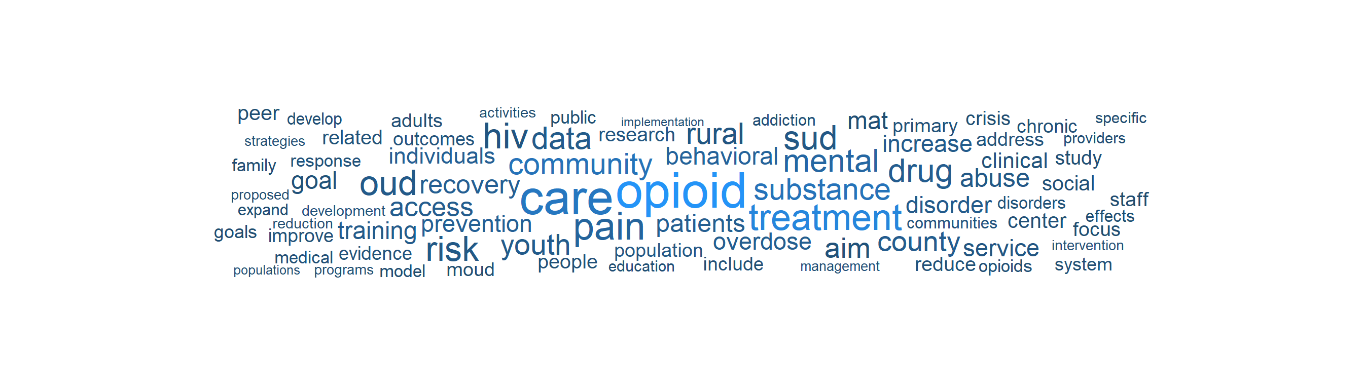
The word cloud below visualizes the most frequent terms appearing in award descriptions across all `r format(nrow(awards), big.mark = ",")` retrieved opioid-related grants. Larger words appear more often, revealing the dominant themes in federal spending. Use the [Drug Overdose Crisis Explorer](https://intersect-collaborations-llc.shinyapps.io/drug-overdose-explorer/) to search, filter, and download the full award dataset.
```{r}
#| label: usaspending-wordcloud
#| eval: true
#| code-fold: true
#| column: page
#| fig-width: 14
#| fig-height: 4
#| out-width: "100%"
# Use the full (untruncated) descriptions from the API response
full_descriptions <- spending_data$results$Description

# Tokenize into individual words, remove stop words and generic terms
word_counts <- tibble(text = full_descriptions) |>
  filter(!is.na(text), text != "") |>
  unnest_tokens(word, text) |>
  anti_join(stop_words, by = "word") |>
  filter(
    !word %in% c("award", "grant", "funding", "program", "provide",
                  "project", "based", "including", "support", "services",
                  "funds", "federal", "national", "department", "health",
                  "1", "2", "3", "4", "5", "01", "02", "12",
                  as.character(year_start:year_end), "cfda", "fy"),
    nchar(word) > 2,
    !grepl("^[0-9]+$", word)
  ) |>
  count(word, sort = TRUE)

ggplot(word_counts |> head(80), aes(label = word, size = n, color = n)) +
  geom_text_wordcloud_area(family = "sans", shape = "square") +
  scale_size_area(max_size = 28) +
  scale_color_gradient(low = "#204d70", high = "#2494f7") +
  theme_minimal() +
  theme(
    plot.background = element_rect(fill = "white", color = NA),
    plot.margin = margin(0, 0, 0, 0)
  )
```
#### Federal Funding Over Time
The chart below plots individual grant award amounts by their start date, colored by awarding sub-agency. Hover over each point to see the recipient and award details.
```{r}
#| label: usaspending-funding-timeline
#| eval: true
#| code-fold: true
# Prepare data for the timeline chart
funding_timeline <- awards |>
  mutate(
    start_date = as.Date(`Start Date`),
    award_amount = as.numeric(`Award Amount`),
    agency = `Awarding Sub Agency`,
    recipient = `Recipient Name`,
    hover_text = paste0(
      "<b>", agency, "</b><br>",
      "Recipient: ", recipient, "<br>",
      "Award: $", formatC(award_amount, format = "f", digits = 0, big.mark = ",")
    )
  ) |>
  filter(!is.na(start_date), !is.na(award_amount))

# Brand-aligned color palette for agencies
agency_colors <- c(
  "#2494f7", "#00a4bb", "#01272f", "#204d70",
  "#e07b39", "#6b4c9a", "#d94f4f", "#2ca02c",
  "#8c564b", "#17becf", "#bcbd22", "#7f7f7f"
)

funding_plot <- plot_ly(
  data = funding_timeline,
  x = ~start_date,
  y = ~award_amount,
  color = ~agency,
  colors = agency_colors,
  type = "scatter",
  mode = "markers",
  marker = list(size = 8, opacity = 0.7),
  text = ~hover_text,
  hoverinfo = "text"
) |>
  layout(
    title = list(
      text = paste0("Opioid-Related Federal Grant Awards Over Time (",
                    year_start, "-", year_end, ")"),
      font = list(size = 16)
    ),
    xaxis = list(
      title = "Award Start Date",
      type = "date"
    ),
    yaxis = list(
      title = "Award Amount ($)",
      separatethousands = TRUE,
      type = "log"
    ),
    legend = list(
      title = list(text = "Awarding Sub Agency"),
      orientation = "h",
      y = -0.25,
      x = 0,
      font = list(size = 9)
    ),
    hovermode = "closest",
    margin = list(b = 120),
    height = 800
  ) |>
  config(displayModeBar = TRUE)

funding_plot
```
#### Total Federal Funding by Agency
The chart below summarizes annual opioid-related grant funding by awarding sub-agency. The stacked bars show each agency's contribution, while the line traces the overall annual total.
```{r}
#| label: usaspending-funding-by-agency
#| eval: true
#| code-fold: true
# Summarize annual funding by sub-agency
funding_by_agency <- awards |>
  mutate(
    start_date = as.Date(`Start Date`),
    start_year = as.integer(format(start_date, "%Y")),
    agency = `Awarding Sub Agency`
  ) |>
  filter(!is.na(start_year), !is.na(award_amount)) |>
  group_by(start_year, agency) |>
  summarise(
    total = sum(award_amount, na.rm = TRUE),
    n_awards = n(),
    .groups = "drop"
  )

# Overall annual totals for the line trace
funding_annual_total <- funding_by_agency |>
  group_by(start_year) |>
  summarise(
    grand_total = sum(total, na.rm = TRUE),
    n_awards = sum(n_awards),
    .groups = "drop"
  )

agency_bar_plot <- plot_ly() |>
  add_trace(
    data = funding_by_agency,
    x = ~start_year,
    y = ~total,
    color = ~agency,
    colors = agency_colors,
    type = "bar",
    text = ~paste0(
      "<b>", agency, "</b><br>",
      "Year: ", start_year, "<br>",
      "Awards: ", n_awards, "<br>",
      "Total: $", formatC(total, format = "f", digits = 0, big.mark = ",")
    ),
    hoverinfo = "text"
  ) |>
  add_trace(
    data = funding_annual_total,
    x = ~start_year,
    y = ~grand_total,
    type = "scatter",
    mode = "lines+markers",
    name = "Annual Total",
    line = list(color = "#020506", width = 3),
    marker = list(color = "#020506", size = 8),
    text = ~paste0(
      "<b>Annual Total</b><br>",
      "Year: ", start_year, "<br>",
      "Awards: ", n_awards, "<br>",
      "Total: $", formatC(grand_total, format = "f", digits = 0, big.mark = ",")
    ),
    hoverinfo = "text"
  ) |>
  layout(
    title = list(
      text = paste0("Total Opioid-Related Federal Grant Funding by Agency (",
                    year_start, "-", year_end, ")"),
      font = list(size = 16)
    ),
    xaxis = list(title = "Year", dtick = 1),
    yaxis = list(title = "Total Funding ($)", separatethousands = TRUE),
    barmode = "stack",
    legend = list(
      title = list(text = "Awarding Sub Agency"),
      orientation = "h",
      y = -0.25, x = 0,
      font = list(size = 9)
    ),
    hovermode = "x unified",
    margin = list(b = 120),
    height = 800
  ) |>
  config(displayModeBar = TRUE)

agency_bar_plot
```
For the full searchable and downloadable award dataset, use the [Drug Overdose Crisis Explorer](https://intersect-collaborations-llc.shinyapps.io/drug-overdose-explorer/).
::: {.callout-note title="Data Source"}
USAspending is the official U.S. government open data source for federal spending. HHS TAGGS provides more granular transaction-level tracking of HHS grant obligations specifically.
:::
## Research Literature and Databases
Beyond surveillance data, a large and growing body of peer-reviewed research examines the epidemiology, pharmacology, policy responses, and social determinants of the overdose crisis. Several public databases allow programmatic access to this literature and to information about funded research projects.
### NIH RePORTER (Funded Research Projects)
[NIH RePORTER](https://reporter.nih.gov/) tracks all NIH-funded research projects, including active grants, publications, patents, and clinical trials. Its [API](https://api.reporter.nih.gov/) supports POST-based queries to identify what research is currently being funded on any topic.
```{r}
#| label: nih-reporter-search
#| eval: true
#| code-fold: true
# NIH RePORTER API: find funded opioid overdose research projects
# Documentation: https://api.reporter.nih.gov/

reporter_url <- "https://api.reporter.nih.gov/v2/projects/search"

# Paginate to collect all available projects
all_projects <- list()
for (pg in 0:99) {
  reporter_body <- list(
    criteria = list(
      advanced_text_search = list(
        operator = "and",
        search_field = "projecttitle,terms",
        search_text = "opioid overdose fentanyl"
      ),
      fiscal_years = as.list((year_end - 4L):year_end),
      exclude_subprojects = TRUE
    ),
    offset = pg * 100,
    limit = 100,
    sort_field = "FiscalYear",
    sort_order = "desc"
  )

  reporter_response <- request(reporter_url) |>
    req_body_json(reporter_body) |>
    req_perform()

  reporter_data <- reporter_response |>
    resp_body_json()

  if (length(reporter_data$results) == 0) break
  all_projects[[pg + 1]] <- reporter_data$results
  if (length(reporter_data$results) < 100) break
}

reporter_total <- reporter_data$meta$total

# Parse all results into a dataframe
projects <- lapply(unlist(all_projects, recursive = FALSE), function(p) {
  tibble(
    project_num   = p$project_num %||% NA_character_,
    fiscal_year   = p$fiscal_year %||% NA_integer_,
    title         = p$project_title %||% NA_character_,
    pi_name       = {
      if (!is.null(p$principal_investigators) && length(p$principal_investigators) > 0)
        p$principal_investigators[[1]]$full_name
      else NA_character_
    },
    organization  = p$organization$org_name %||% NA_character_,
    ic_name       = {
      ics <- p$agency_ic_fundings
      if (!is.null(ics) && length(ics) > 0) ics[[1]]$abbreviation %||% NA_character_
      else NA_character_
    },
    award_amount  = p$award_amount %||% NA_real_,
    abstract_text = p$abstract_text %||% NA_character_
  )
}) |>
  bind_rows()
```
The search matched **`r format(reporter_total, big.mark = ",")`** projects. **`r format(nrow(projects), big.mark = ",")`** were retrieved, representing **$`r format(sum(projects$award_amount, na.rm = TRUE), big.mark = ",")`** in total funding.
#### NIH Project Awards Over Time
The chart below plots individual NIH-funded project award amounts by fiscal year, colored by NIH Institute/Center (IC). Hover over each point to see the project title, PI, and award amount.
```{r}
#| label: nih-reporter-scatter
#| eval: true
#| code-fold: true
library(plotly)

nih_scatter_df <- projects |>
  filter(!is.na(award_amount), !is.na(fiscal_year)) |>
  mutate(
    ic_label = ifelse(is.na(ic_name), "Other", ic_name),
    hover_text = paste0(
      "<b>", ic_label, "</b><br>",
      "PI: ", pi_name, "<br>",
      "Title: ", substr(title, 1, 80), "<br>",
      "Award: $", formatC(award_amount, format = "f", digits = 0, big.mark = ",")
    )
  )

ic_colors <- c(
  "#2494f7", "#00a4bb", "#01272f", "#204d70",
  "#e07b39", "#6b4c9a", "#d94f4f", "#2ca02c",
  "#8c564b", "#17becf", "#bcbd22", "#7f7f7f"
)

nih_scatter_plot <- plot_ly(
  data = nih_scatter_df,
  x = ~fiscal_year,
  y = ~award_amount,
  color = ~ic_label,
  colors = ic_colors,
  type = "scatter",
  mode = "markers",
  marker = list(size = 8, opacity = 0.7),
  text = ~hover_text,
  hoverinfo = "text"
) |>
  layout(
    title = list(
      text = paste0("NIH Opioid Research Project Awards (",
                    year_end - 4, "-", year_end, ")"),
      font = list(size = 16)
    ),
    xaxis = list(title = "Fiscal Year", dtick = 1),
    yaxis = list(
      title = "Award Amount ($)",
      separatethousands = TRUE,
      type = "log"
    ),
    legend = list(
      title = list(text = "NIH Institute/Center"),
      orientation = "h",
      y = -0.25, x = 0,
      font = list(size = 9)
    ),
    hovermode = "closest",
    margin = list(b = 120),
    height = 800
  ) |>
  config(displayModeBar = TRUE)

nih_scatter_plot
```
#### NIH Funding by Institute/Center
The stacked bar chart below summarizes annual NIH opioid research funding by Institute/Center. The line traces the overall annual total.
```{r}
#| label: nih-reporter-timeline
#| eval: true
#| code-fold: true
# Summarize funding by fiscal year and IC
nih_by_ic <- projects |>
  filter(!is.na(award_amount), !is.na(fiscal_year)) |>
  mutate(ic_label = ifelse(is.na(ic_name), "Other", ic_name)) |>
  group_by(fiscal_year, ic_label) |>
  summarise(
    total = sum(award_amount, na.rm = TRUE),
    n_projects = n(),
    .groups = "drop"
  )

nih_annual_total <- nih_by_ic |>
  group_by(fiscal_year) |>
  summarise(
    grand_total = sum(total, na.rm = TRUE),
    n_projects = sum(n_projects),
    .groups = "drop"
  )

nih_timeline_plot <- plot_ly() |>
  add_trace(
    data = nih_by_ic,
    x = ~fiscal_year,
    y = ~total,
    color = ~ic_label,
    colors = ic_colors,
    type = "bar",
    text = ~paste0(
      "<b>", ic_label, "</b><br>",
      "FY ", fiscal_year, "<br>",
      "Projects: ", n_projects, "<br>",
      "Total: $", formatC(total, format = "f", digits = 0, big.mark = ",")
    ),
    hoverinfo = "text"
  ) |>
  add_trace(
    data = nih_annual_total,
    x = ~fiscal_year,
    y = ~grand_total,
    type = "scatter",
    mode = "lines+markers",
    name = "Annual Total",
    line = list(color = "#020506", width = 3),
    marker = list(color = "#020506", size = 8),
    text = ~paste0(
      "<b>Annual Total</b><br>",
      "FY ", fiscal_year, "<br>",
      "Projects: ", n_projects, "<br>",
      "Total: $", formatC(grand_total, format = "f", digits = 0, big.mark = ",")
    ),
    hoverinfo = "text"
  ) |>
  layout(
    title = list(
      text = "NIH Opioid Overdose Research Funding by Fiscal Year and IC",
      font = list(size = 16)
    ),
    xaxis = list(title = "Fiscal Year", dtick = 1),
    yaxis = list(title = "Total Award Amount ($)", separatethousands = TRUE),
    barmode = "stack",
    legend = list(
      title = list(text = "NIH Institute/Center"),
      orientation = "h",
      y = -0.25, x = 0,
      font = list(size = 9)
    ),
    hovermode = "x unified",
    margin = list(b = 120),
    height = 800
  ) |>
  config(displayModeBar = TRUE)

nih_timeline_plot
```
#### What Is NIH Funding?
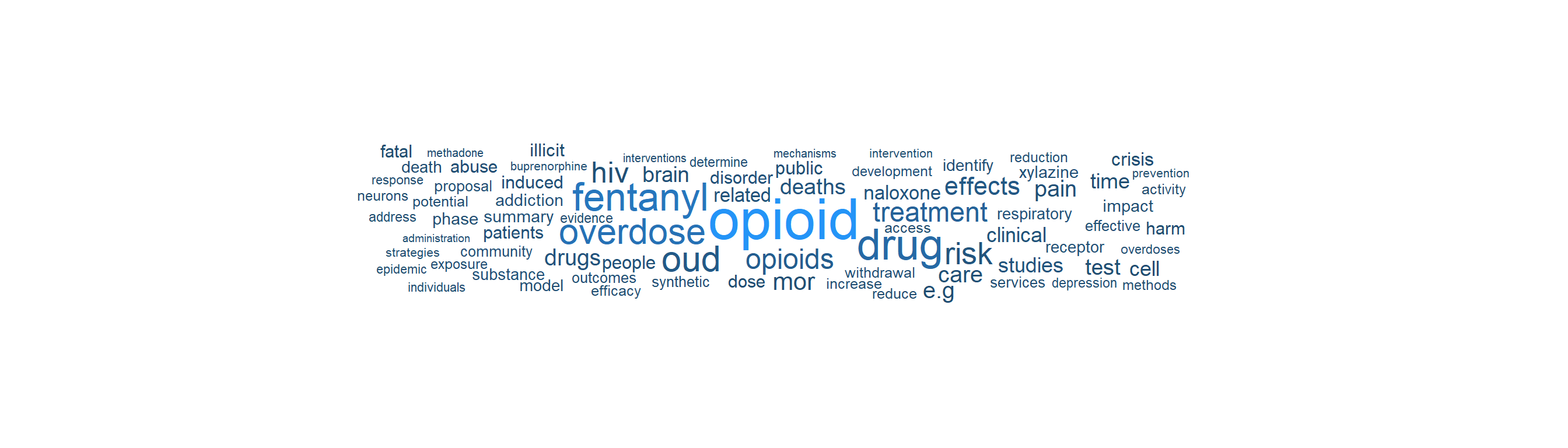
The word cloud below visualizes the most frequent terms appearing in project abstracts across all `r nrow(projects)` retrieved NIH-funded opioid research projects, revealing the dominant research themes. Use the [Drug Overdose Crisis Explorer](https://intersect-collaborations-llc.shinyapps.io/drug-overdose-explorer/) to search, filter, and download the full project dataset.
```{r}
#| label: nih-reporter-wordcloud
#| eval: true
#| code-fold: true
#| column: page
#| fig-width: 14
#| fig-height: 4
#| out-width: "100%"
# Tokenize abstracts into individual words, remove stop words and generic terms
nih_word_counts <- tibble(text = projects$abstract_text) |>
  filter(!is.na(text), text != "") |>
  unnest_tokens(word, text) |>
  anti_join(stop_words, by = "word") |>
  filter(
    !word %in% c("study", "research", "project", "aim", "aims",
                  "specific", "propose", "proposed", "will", "use",
                  "data", "based", "including", "provide", "develop",
                  "support", "national", "health", "program", "grant",
                  "funding", "abstract", "1", "2", "3", "4", "5",
                  "r01", "r21", "r34", "k01", "k23", "u01", "p50"),
    nchar(word) > 2,
    !grepl("^[0-9]+$", word)
  ) |>
  count(word, sort = TRUE)

ggplot(nih_word_counts |> head(80), aes(label = word, size = n, color = n)) +
  geom_text_wordcloud_area(family = "sans", shape = "square") +
  scale_size_area(max_size = 28) +
  scale_color_gradient(low = "#204d70", high = "#2494f7") +
  theme_minimal() +
  theme(
    plot.background = element_rect(fill = "white", color = NA),
    plot.margin = margin(0, 0, 0, 0)
  )
```
#### Highest-Funded Projects
The table below shows the five largest NIH-funded opioid overdose research projects by award amount. For the full searchable and downloadable project dataset, use the [Drug Overdose Crisis Explorer](https://intersect-collaborations-llc.shinyapps.io/drug-overdose-explorer/).
```{r}
#| label: nih-reporter-table
#| eval: true
#| code-fold: true
projects |>
  arrange(desc(award_amount)) |>
  head(5) |>
  select(
    `Project Number` = project_num,
    `Fiscal Year` = fiscal_year,
    Title = title, PI = pi_name,
    Organization = organization,
    `Award Amount` = award_amount
  ) |>
  knitr::kable(
    format.args = list(big.mark = ","),
    caption = paste0(
      "Top 5 NIH-Funded Opioid Overdose Research Projects by Award Amount (",
      year_end - 4, "-", year_end, ")"
    )
  )
```
::: {.callout-note title="Data Source"}
NIH RePORTER is the authoritative source for federally funded biomedical research. It covers grants from NIH, CDC, FDA, AHRQ, SAMHSA, and other HHS agencies. No authentication is required. The API returns project details, funding amounts, and links to resulting publications.
:::
### ClinicalTrials.gov (Clinical Research)
[ClinicalTrials.gov](https://clinicaltrials.gov/) registers clinical studies on a wide range of conditions, including opioid use disorder treatment trials, naloxone distribution studies, and harm reduction interventions. The [v2 API](https://clinicaltrials.gov/data-api/about-api) supports structured queries.
```{r}
#| label: clinicaltrials-search
#| eval: true
#| code-fold: true
# ClinicalTrials.gov v2 API: find opioid-related clinical trials
# Documentation: https://clinicaltrials.gov/data-api/about-api
# Paginate using nextPageToken to collect up to ~200 trials

ct_url <- "https://clinicaltrials.gov/api/v2/studies"

all_trials_raw <- list()
next_token <- NULL
for (pg in 1:10) {
  ct_query <- list(
    `query.cond`  = "opioid overdose",
    `query.intr`  = "fentanyl OR naloxone OR buprenorphine",
    `filter.overallStatus` = "RECRUITING,ACTIVE_NOT_RECRUITING,COMPLETED",
    countTotal    = "true",
    pageSize      = 100,
    sort          = "LastUpdatePostDate:desc"
  )
  if (!is.null(next_token)) ct_query$pageToken <- next_token

  ct_response <- request(ct_url) |>
    req_url_query(!!!ct_query) |>
    req_perform()

  ct_data <- ct_response |>
    resp_body_json()

  if (length(ct_data$studies) == 0) break
  all_trials_raw[[pg]] <- ct_data$studies
  next_token <- ct_data$nextPageToken
  if (is.null(next_token)) break
}

ct_total <- ct_data$totalCount

trials <- lapply(unlist(all_trials_raw, recursive = FALSE), function(s) {
  proto <- s$protocolSection
  id_mod <- proto$identificationModule
  status_mod <- proto$statusModule
  sponsor_mod <- proto$sponsorCollaboratorsModule
  design_mod <- proto$designModule
  desc_mod <- proto$descriptionModule

  tibble(
    nct_id      = id_mod$nctId %||% NA_character_,
    title       = id_mod$briefTitle %||% NA_character_,
    status      = status_mod$overallStatus %||% NA_character_,
    start_date  = status_mod$startDateStruct$date %||% NA_character_,
    sponsor     = sponsor_mod$leadSponsor$name %||% NA_character_,
    enrollment  = design_mod$enrollmentInfo$count %||% NA_integer_,
    description = desc_mod$briefSummary %||% NA_character_
  )
}) |>
  bind_rows()
```
The search matched **`r format(ct_total, big.mark = ",")`** studies. **`r nrow(trials)`** trials were retrieved for analysis.
#### Clinical Trials Over Time
The chart below shows the number of opioid-related clinical trials by their start year, broken down by status.
```{r}
#| label: clinicaltrials-timeline
#| eval: true
#| code-fold: true
library(plotly)

trials_timeline <- trials |>
  mutate(
    start_year = as.integer(substr(start_date, 1, 4))
  ) |>
  filter(!is.na(start_year)) |>
  count(start_year, status, name = "n_trials") |>
  arrange(start_year)

# Brand-aligned status colors
status_colors <- c(
  "COMPLETED" = "#2494f7",
  "ACTIVE_NOT_RECRUITING" = "#00a4bb",
  "RECRUITING" = "#204d70"
)

ct_timeline_plot <- plot_ly(
  data = trials_timeline,
  x = ~start_year,
  y = ~n_trials,
  color = ~status,
  colors = status_colors,
  type = "bar",
  text = ~paste0(
    "<b>", start_year, "</b><br>",
    status, ": ", n_trials, " trials"
  ),
  hoverinfo = "text"
) |>
  layout(
    title = list(
      text = "Opioid-Related Clinical Trials by Start Year and Status",
      font = list(size = 16)
    ),
    xaxis = list(title = "Start Year", dtick = 1),
    yaxis = list(title = "Number of Trials"),
    barmode = "stack",
    legend = list(
      title = list(text = "Trial Status"),
      orientation = "h",
      y = -0.2, x = 0
    ),
    hovermode = "x unified"
  ) |>
  config(displayModeBar = TRUE)

ct_timeline_plot
```
#### Clinical Trial Research Themes
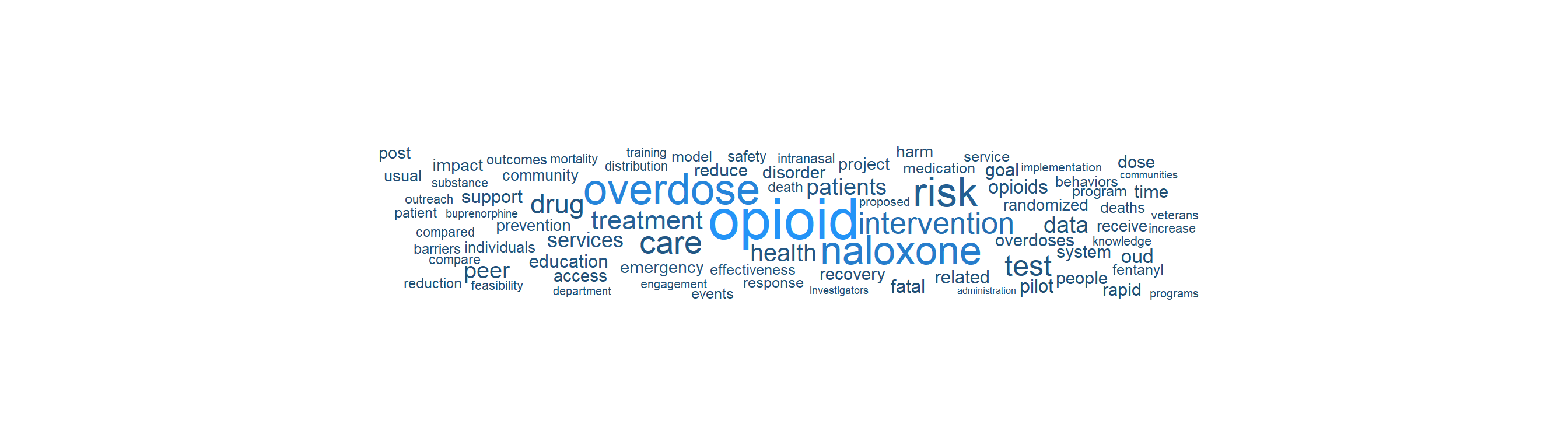
The word cloud below visualizes the most frequent terms in trial titles and descriptions, revealing the dominant intervention and population themes in clinical research. Use the [Drug Overdose Crisis Explorer](https://intersect-collaborations-llc.shinyapps.io/drug-overdose-explorer/) to search, filter, and download the full trial dataset.
```{r}
#| label: clinicaltrials-wordcloud
#| eval: true
#| code-fold: true
#| column: page
#| fig-width: 14
#| fig-height: 4
#| out-width: "100%"
ct_word_counts <- trials |>
  mutate(text = paste(title, description, sep = " ")) |>
  select(text) |>
  filter(!is.na(text), text != " ") |>
  unnest_tokens(word, text) |>
  anti_join(stop_words, by = "word") |>
  filter(
    !word %in% c("study", "trial", "clinical", "phase",
                  "participants", "purpose", "determine",
                  "evaluate", "assess", "including", "based",
                  "aims", "aim", "objective", "primary"),
    nchar(word) > 2,
    !grepl("^[0-9]+$", word)
  ) |>
  count(word, sort = TRUE)

ggplot(ct_word_counts |> head(80), aes(label = word, size = n, color = n)) +
  geom_text_wordcloud_area(family = "sans", shape = "square") +
  scale_size_area(max_size = 28) +
  scale_color_gradient(low = "#204d70", high = "#2494f7") +
  theme_minimal() +
  theme(
    plot.background = element_rect(fill = "white", color = NA),
    plot.margin = margin(0, 0, 0, 0)
  )
```
#### Most Recent Trials
The table below shows the five most recently started opioid overdose intervention trials. For the full searchable and downloadable trial dataset, use the [Drug Overdose Crisis Explorer](https://intersect-collaborations-llc.shinyapps.io/drug-overdose-explorer/).
```{r}
#| label: clinicaltrials-table
#| eval: true
#| code-fold: true
trials |>
  arrange(desc(start_date)) |>
  head(5) |>
  select(
    `NCT ID` = nct_id, Title = title, Status = status,
    `Start Date` = start_date, Sponsor = sponsor,
    Enrollment = enrollment
  ) |>
  knitr::kable(
    format.args = list(big.mark = ","),
    caption = "5 Most Recent Opioid Overdose Intervention Trials"
  )
```
::: {.callout-tip title="Reproducibility"}
ClinicalTrials.gov does not require authentication. The v2 API returns JSON by default and supports filtering by condition, intervention, status, location, and date range. This is useful for mapping the research landscape around specific interventions (e.g., naloxone distribution, buprenorphine access).
:::
### PubMed (NCBI E-utilities API)
[PubMed](https://pubmed.ncbi.nlm.nih.gov/) indexes over 37 million biomedical citations. The [NCBI E-utilities API](https://www.ncbi.nlm.nih.gov/books/NBK25501/) enables programmatic search and retrieval without authentication (subject to rate limits of 3 requests per second without an API key, or 10 per second with one).
```{r}
#| label: pubmed-search
#| eval: true
library(httr2)
library(jsonlite)
library(dplyr)
library(tidyr)

# NCBI E-utilities: search PubMed for recent opioid overdose research
# Documentation: https://www.ncbi.nlm.nih.gov/books/NBK25501/

# Step 1: Search for article IDs matching our query
esearch_url <- "https://eutils.ncbi.nlm.nih.gov/entrez/eutils/esearch.fcgi"

search_response <- request(esearch_url) |>
  req_url_query(
    db       = "pubmed",
    term     = "opioid overdose fentanyl United States[Title/Abstract]",
    retmax   = 10000,
    sort     = "date",
    retmode  = "json",
    mindate  = format(date_start, "%Y/%m/%d"),
    maxdate  = format(date_end, "%Y/%m/%d"),
    datetype = "pdat"
  ) |>
  req_perform()

search_results <- search_response |>
  resp_body_json()

# Extract PubMed IDs
pmids <- search_results$esearchresult$idlist

# Step 2: Fetch article summaries for those IDs
esummary_url <- "https://eutils.ncbi.nlm.nih.gov/entrez/eutils/esummary.fcgi"

if (length(pmids) > 0) {
  summary_response <- request(esummary_url) |>
    req_url_query(
      db      = "pubmed",
      id      = paste(pmids, collapse = ","),
      retmode = "json"
    ) |>
    req_perform()

  summaries <- summary_response |>
    resp_body_json()

  # Parse into a tidy dataframe
  articles <- lapply(pmids, function(id) {
    article <- summaries$result[[id]]
    tibble(
      pmid      = id,
      title     = article$title %||% NA_character_,
      journal   = article$fulljournalname %||% NA_character_,
      pub_date  = article$pubdate %||% NA_character_,
      doi       = {
        doi_ids <- Filter(function(x) x$idtype == "doi", article$articleids)
        if (length(doi_ids) > 0) doi_ids[[1]]$value else NA_character_
      }
    )
  }) |>
    bind_rows()
}
```
The search matched **`r format(as.integer(search_results$esearchresult$count), big.mark = ",")`** articles. **`r nrow(articles)`** were retrieved for analysis.
#### Publication Trends Over Time
The chart below shows the volume of opioid overdose fentanyl research published over time. Each point represents the number of articles published in a given month.
```{r}
#| label: pubmed-timeline
#| eval: true
#| code-fold: true
library(plotly)
library(lubridate)

# Parse publication dates into proper Date objects
# PubMed dates come in formats like "2025 Jan 15", "2025 Mar", "2025"
pubmed_timeline <- articles |>
  mutate(
    pub_date_parsed = case_when(
      grepl("^\\d{4} \\w+ \\d+", pub_date) ~
        as.Date(pub_date, format = "%Y %b %d"),
      grepl("^\\d{4} \\w+", pub_date) ~
        as.Date(paste0(pub_date, " 01"), format = "%Y %b %d"),
      grepl("^\\d{4}$", pub_date) ~
        as.Date(paste0(pub_date, " Jan 01"), format = "%Y %b %d"),
      TRUE ~ NA_Date_
    ),
    pub_month = floor_date(pub_date_parsed, "month")
  ) |>
  filter(!is.na(pub_month))

# Count articles per month
monthly_counts <- pubmed_timeline |>
  count(pub_month, name = "n_articles") |>
  arrange(pub_month)

# Interactive time series
pubmed_plot <- plot_ly(
  data = monthly_counts,
  x = ~pub_month,
  y = ~n_articles,
  type = "scatter",
  mode = "lines+markers",
  line = list(color = "#2494f7", width = 2),
  marker = list(color = "#2494f7", size = 6),
  hovertemplate = paste(
    "<b>%{x|%B %Y}</b><br>",
    "Articles: %{y}<extra></extra>"
  )
) |>
  layout(
    title = list(
      text = "Opioid Overdose Fentanyl Research: Publications per Month",
      font = list(size = 16)
    ),
    xaxis = list(
      title = "Publication Month",
      type = "date",
      rangeslider = list(visible = TRUE)
    ),
    yaxis = list(
      title = "Number of Articles"
    ),
    hovermode = "x unified"
  ) |>
  config(displayModeBar = TRUE)

pubmed_plot
```
#### Research Themes in Article Titles
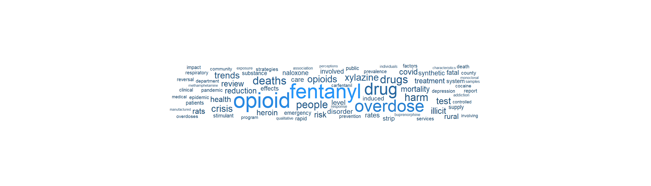
The word cloud below visualizes the most frequent terms appearing in the titles of all `r nrow(articles)` retrieved PubMed articles. This provides a quick thematic overview of the research landscape. Use the [Drug Overdose Crisis Explorer](https://intersect-collaborations-llc.shinyapps.io/drug-overdose-explorer/) to search, filter, and download the full publication dataset.
```{r}
#| label: pubmed-wordcloud
#| eval: true
#| code-fold: true
#| column: page
#| fig-width: 14
#| fig-height: 4
#| out-width: "100%"
# Tokenize article titles into individual words
pubmed_title_words <- tibble(text = articles$title) |>
  filter(!is.na(text), text != "") |>
  unnest_tokens(word, text) |>
  anti_join(stop_words, by = "word") |>
  filter(
    !word %in% c("study", "analysis", "among", "associated",
                  "united", "states", "results", "based",
                  "findings", "using", "related", "data"),
    nchar(word) > 2,
    !grepl("^[0-9]+$", word)
  ) |>
  count(word, sort = TRUE)

ggplot(pubmed_title_words |> head(80), aes(label = word, size = n, color = n)) +
  geom_text_wordcloud_area(family = "sans", shape = "square") +
  scale_size_area(max_size = 28) +
  scale_color_gradient(low = "#204d70", high = "#2494f7") +
  theme_minimal() +
  theme(
    plot.background = element_rect(fill = "white", color = NA),
    plot.margin = margin(0, 0, 0, 0)
  )
```
#### Most Recent Publications
The table below shows the five most recently published opioid overdose fentanyl articles indexed in PubMed. For the full searchable and downloadable publication dataset, use the [Drug Overdose Crisis Explorer](https://intersect-collaborations-llc.shinyapps.io/drug-overdose-explorer/).
```{r}
#| label: pubmed-article-table
#| eval: true
#| code-fold: true
articles |>
  arrange(desc(pub_date)) |>
  head(5) |>
  select(
    PMID = pmid, Title = title, Journal = journal,
    `Publication Date` = pub_date
  ) |>
  knitr::kable(
    caption = paste0(
      "5 Most Recent PubMed Articles: Opioid Overdose Fentanyl Research (",
      format(date_start, "%Y"), "-", format(date_end, "%Y"), ")"
    )
  )
```
::: {.callout-tip title="Reproducibility"}
For higher rate limits, register for a free NCBI API key at [ncbi.nlm.nih.gov/account](https://www.ncbi.nlm.nih.gov/account/) and append `&api_key=YOUR_KEY` to requests. The E-utilities support complex Boolean queries using MeSH terms (e.g., `"Opiate Overdose"[MeSH] AND "Fentanyl"[MeSH]`) for more precise results.
:::
### Europe PMC (Open Access Literature)
[Europe PMC](https://europepmc.org/) provides open access to a worldwide collection of life science publications, including all PubMed content plus preprints, patents, and clinical guidelines. Its [REST API](https://europepmc.org/RestfulWebService) is particularly useful for retrieving full-text open access articles.
```{r}
#| label: europe-pmc-search
#| eval: true
#| code-fold: true
# Paginate to collect all available results (pageSize max is 1000)

epmc_url <- "https://www.ebi.ac.uk/europepmc/webservices/rest/search"

epmc_all <- list()
for (pg in 1:50) {
  epmc_response <- request(epmc_url) |>
    req_url_query(
      query      = paste0("(opioid overdose fentanyl) AND (PUB_YEAR:[",
                          year_start, " TO ", year_end, "])"),
      format     = "json",
      pageSize   = 1000,
      cursorMark = if (pg == 1) "*" else epmc_cursor,
      resultType = "core"
    ) |>
    req_perform()

  epmc_data <- epmc_response |>
    resp_body_json()

  if (length(epmc_data$resultList$result) == 0) break
  epmc_all[[pg]] <- epmc_data$resultList$result
  epmc_cursor <- epmc_data$nextCursorMark %||% NULL
  if (is.null(epmc_cursor) || length(epmc_data$resultList$result) < 1000) break
}

epmc_hit_count <- epmc_data$hitCount

epmc_articles <- lapply(unlist(epmc_all, recursive = FALSE), function(a) {
  tibble(
    pmid            = a$pmid %||% NA_character_,
    title           = a$title %||% NA_character_,
    journal         = a$journalTitle %||% NA_character_,
    year            = a$pubYear %||% NA_character_,
    first_pub_date  = a$firstPublicationDate %||% NA_character_,
    is_open_access  = a$isOpenAccess %||% "N",
    cited_by_count  = a$citedByCount %||% 0L,
    doi             = a$doi %||% NA_character_,
    abstract        = a$abstractText %||% NA_character_
  )
}) |>
  bind_rows()
```
The search matched **`r format(epmc_hit_count, big.mark = ",")`** results. **`r format(nrow(epmc_articles), big.mark = ",")`** articles were retrieved, of which **`r sum(epmc_articles$is_open_access == "Y", na.rm = TRUE)`** are open access.
#### Europe PMC: Publication Timeline
The chart below shows the volume of opioid overdose fentanyl research indexed in Europe PMC by publication year.
```{r}
#| label: europe-pmc-timeline
#| eval: true
#| code-fold: true
library(plotly)

epmc_by_year <- epmc_articles |>
  filter(!is.na(.data$year)) |>
  mutate(pub_year = as.integer(.data$year)) |>
  count(pub_year, name = "n_articles") |>
  arrange(pub_year)

epmc_timeline_plot <- plot_ly(
  data = epmc_by_year,
  x = ~pub_year,
  y = ~n_articles,
  type = "bar",
  marker = list(color = "#00a4bb"),
  text = ~paste0("<b>", pub_year, "</b><br>Articles: ", n_articles),
  hoverinfo = "text"
) |>
  layout(
    title = list(
      text = "Europe PMC: Opioid Overdose Fentanyl Publications by Year",
      font = list(size = 16)
    ),
    xaxis = list(title = "Publication Year", dtick = 1),
    yaxis = list(title = "Number of Articles"),
    hovermode = "x unified"
  ) |>
  config(displayModeBar = TRUE)

epmc_timeline_plot
```
#### Europe PMC: Research Themes
The word cloud below visualizes the most frequent terms in article titles and abstracts retrieved from Europe PMC. Use the [Drug Overdose Crisis Explorer](https://intersect-collaborations-llc.shinyapps.io/drug-overdose-explorer/) to search, filter, and download the full article dataset.
```{r}
#| label: europe-pmc-wordcloud
#| eval: true
#| code-fold: true
#| column: page
#| fig-width: 14
#| fig-height: 4
#| out-width: "100%"
epmc_word_counts <- epmc_articles |>
  mutate(text = paste(title, abstract, sep = " ")) |>
  select(text) |>
  filter(!is.na(text), text != " ") |>
  unnest_tokens(word, text) |>
  anti_join(stop_words, by = "word") |>
  filter(
    !word %in% c("study", "results", "background", "methods",
                  "conclusions", "objective", "purpose", "findings",
                  "data", "based", "including", "conclusion",
                  "aim", "abstract", "introduction"),
    nchar(word) > 2,
    !grepl("^[0-9]+$", word)
  ) |>
  count(word, sort = TRUE)

ggplot(epmc_word_counts |> head(80), aes(label = word, size = n, color = n)) +
  geom_text_wordcloud_area(family = "sans", shape = "square") +
  scale_size_area(max_size = 28) +
  scale_color_gradient(low = "#204d70", high = "#2494f7") +
  theme_minimal() +
  theme(
    plot.background = element_rect(fill = "white", color = NA),
    plot.margin = margin(0, 0, 0, 0)
  )
```
#### Most-Cited Articles
The table below shows the five most-cited opioid overdose fentanyl articles indexed in Europe PMC. For the full searchable and downloadable article dataset, use the [Drug Overdose Crisis Explorer](https://intersect-collaborations-llc.shinyapps.io/drug-overdose-explorer/).
```{r}
#| label: europe-pmc-table
#| eval: true
#| code-fold: true
epmc_articles |>
  mutate(
    `Open Access` = ifelse(is_open_access == "Y", "Yes", "No"),
    `Cited By` = as.integer(cited_by_count)
  ) |>
  arrange(desc(`Cited By`)) |>
  head(5) |>
  select(
    PMID = pmid, Title = title, Journal = journal,
    Year = year, `Open Access`, `Cited By`
  ) |>
  knitr::kable(
    caption = paste0(
      "Top 5 Most-Cited Articles: Opioid Overdose Fentanyl Research (",
      year_start, "-", year_end, ")"
    )
  )
```
# References